Introduction
Face alignment is the task of finding a semantic face shape from an image of human face. The face shape can be defined as a shape vector $S = \{\mathbf p_1, \mathbf p_2, \ldots, \mathbf p_n\}$ containing $n$ semantically interesting spots, i.e. landmarks, such as eye corners, nose tip, mouth corners and face contour, etc.
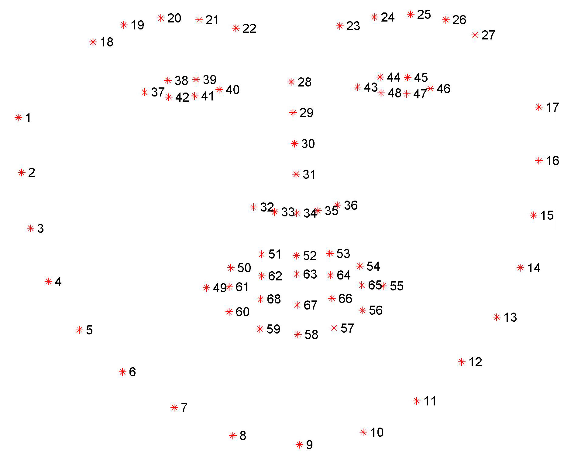
Figure 1. A face shape with 68 landmarks.
Numerous methods have been proposed for face alignment, most of which can be classified into either optimization-based techniques, such as Active Appearance Model, or regression-based techniques such as Explicit Shape Regression.
In this project, a regression based face alignment algorithm, Face Alignment by Explicit Shape Regression, is implemented. This algorithm is one of the state-of-the-art techniques for face alignment that has both high precision and good running time performance.
Algorithm Outline
The explicit shape regression (ESR) algorithm generates face shape by repeatedly refining an initial guess shape via a series of cascaded regression functions. The refinement using a regression function $R$ is called a stage, and there are in total $T$ stages. In each stage $t$, the output of the previous stage, $S^{t-1}$, together with the input image $I$ are used to predict a difference shape $\Delta S^t$. The sum of the difference shape and the current guess shape is the output of stage $t$, i.e.
\[S^t = S^{t-1} + R^{t-1}(I, S^{t-1})\] where $t\in[1..T]$ is the stage index.In each stage, the regression function is computed by minimizing the following error function: \[R^t = \arg\min_R\sum_{i=1}^N\|\hat S_i - (S_i^{t-1}+R(I_i, S_i^{t-1}))\|^2\] where $N$ is the number of training samples.
The regression functions are represented by a series of weak regressors, i.e. \[R^t = (r_1, r_2, \ldots, r_k)\] where each $r_j$ is called a primitive regressor. In each stage, the input shape is refined by all the primitive regressors in a cascaded manner: $k$ primitive regressors form a chain of regressors, where each primitive regressor is called a level. The level $k$ regressor takes the output shape of previous level as input and predict a delta shape vector to refine the input shape vector. The refined shape vector is then passed to the next level of regressor for further refinement.
Typically hundreds of primitive regressors are used in each stage. The primitive regressors are weak regressors because they are only able to reduce the shape error slightly, therefore a series of many primitive regressors are needed in each stage. That said, each primitive regressor alone is not able to reduce the shape error much, but all the primitive regressors collectively are able to reduce the shape error significantly. With enough number of primitive regressors, the final regression function becomes very powerful.
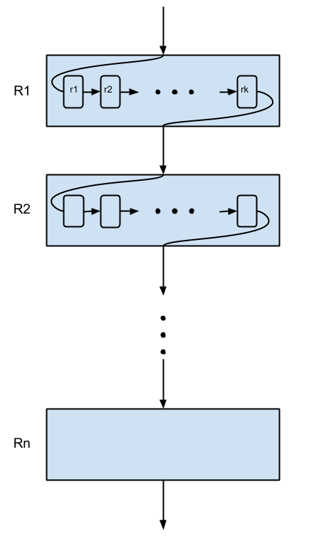
Figure 2. Illustration of the regression function. A regressor function has $n$ stages, and each stage contains $k$ primitive regressors. The guess shape is refined by all primitive regressors in a cascaded manner.
Ferns are chosen as the primitive regressors. A fern is a classification based regressor that takes an $F$ dimensional input feature vector and computes an output vector by classifiy the input into one of the $2^F$ bins. The classification is performed by comparing the input feature vector to $F$ thresholds of the fern. The classification result is an $F$ dimensional binary vector $\mathbf f = (f_1, f_2, \ldots, f_F)$ such that $f_i = 0$ if the $i$th attribute greater than the corresponding threshold and $f_i = 1$ otherwise. The output of the regressor is determined by looking up the output entry for the classification vector.
The output vector for each bin of a fern is computed as \[\delta S_b = \arg\min_{\delta S}\sum_{i\in \Omega_b}\|\hat S_i - (S_i+\delta S)\|\] where $\Omega_b$ is the set of training samples in bin $b$. This gives the following equation of computing the fern output: \[\delta S_b = \frac{\sum_{i\in\Omega_b}(\hat S_i - S_i)}{|\Omega_b|}\] A shrinkage parameter $\beta$ is added to the above equation to overcome over-fitting when the number of training samples in a bin is too small: \[\delta S_b = \frac{1}{1+\beta |\Omega_b|}\frac{\sum_{i\in\Omega_b}(\hat S_i - S_i)}{|\Omega_b|}\]
Implementation Details
Face Detection
The first step of face alignment is to detect face in input images. This is done by using OpenCV face detector. The detector returns a list of bounding boxes of potential face regions, in which the initial guess face shapes are placed.
Face Region Scaling
The input images are scaled according to the detected face regions. The scaling is necessary for achieving stable results because the shape indexed features are sampled directly from input images using given shape indexed locations. Larger face shapes are thus more prone to pixel noise in the images. Scaling the images to make sure the faces in all training samples have similar size reduces the undesired noise. In my implementation, the images are scaled such that the size of detected face region is 128x128.
Training Data
The data used for training is available here. It is a combination of the widely used LFW dataset, LFPW dataset and Helen dataset. All images are annotated with 68 landmarks illustrated in Figure. 1
Face Alignment Procedure
While applying the trained model for face alignment, a random shape vector is chosen from a database of face shapes as initial guess. Since the output of the algorithm is a refinement of the input shape, the quality of the initial guess would inevitably affect the alignment output. To remove the effect of this randomness, multiple initial shapes are used simultaneously and the final shape is computed as a combination of all outputs. Cao et al suggested 5 initial shapes would produce good result in most cases, however, more initial shapes are needed in my experiment.Results and Analysis
Performance Summary
The algorithm is tested with the test data obtain from the same source as training data. The error of the test cases is measured as the mean distance between the output shape vector and the ground truth shape. To obtain a shape invariant measure, the error is normalized by the distance between two pupils of the ground truth shape. For the test data with 507 images, the average normalized error in the test data set is 0.0581, which is comparable to the results reported in [2]. The cumulative error curve of the test data set is shown in Figure 3. Note that the relative error is below 0.1 in more than 90% percent of all test cases, and below 0.05 in about 50% of all test cases.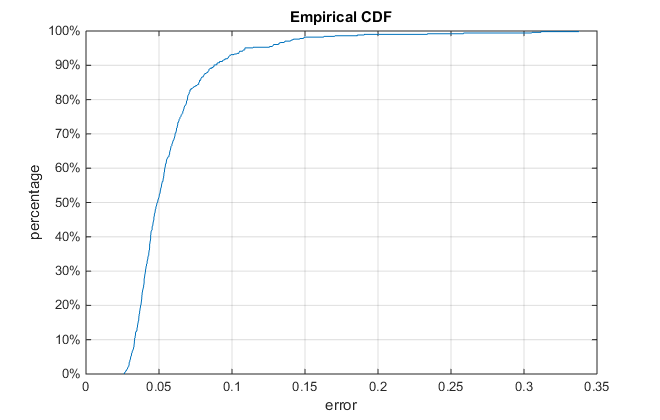
Figure 3. Cumulative error curve of the test data.
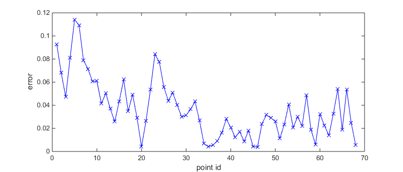
Figure 4. Error curve of a single output shape vector. Figure 5 visualize this shape and corresponding ground truth shape.
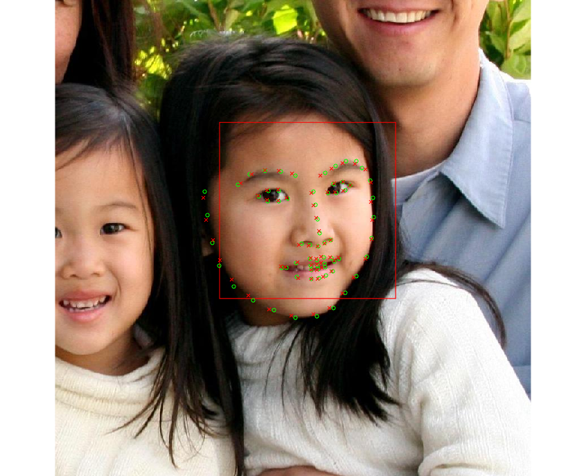
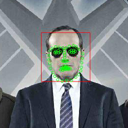
Figure 5. Comparison of output shape (green) and ground truth shape (red).
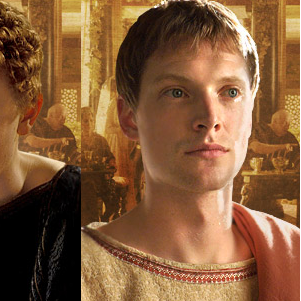
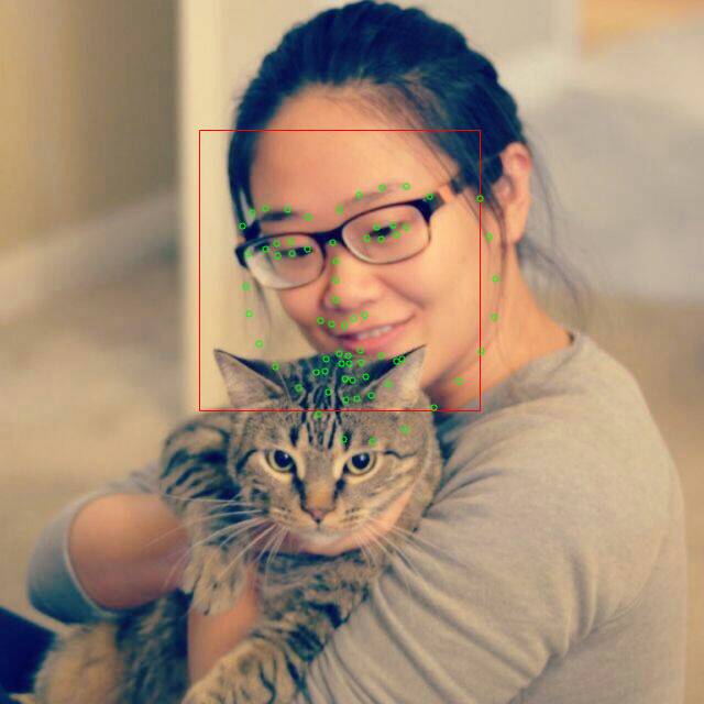
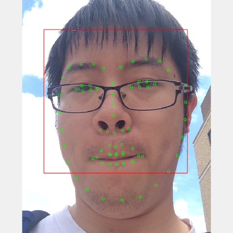
Successful Cases
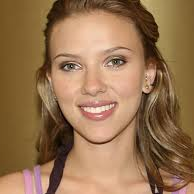
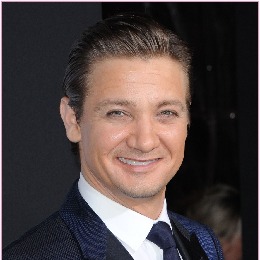
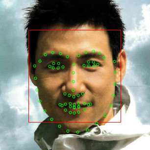
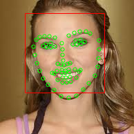
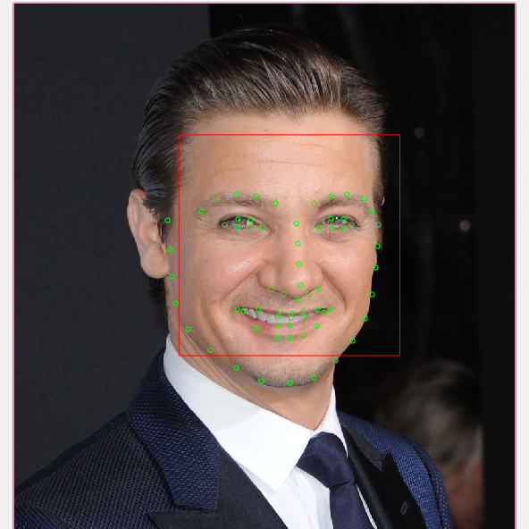
For most images with frontal face and neutral expression, the algorithm works very well. Below are 4 successful cases from the test data. Note the head poses and expressions vary among these images. |
 |
 |
 |
 |
 |
 |
 |
| Succeeded case 1 | Succeeded case 2 | Succeeded case 3 | Succeeded case 4 |
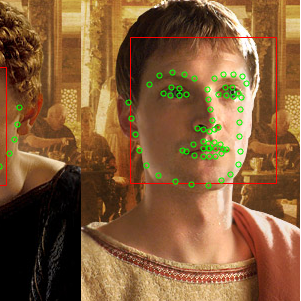
Failed Cases
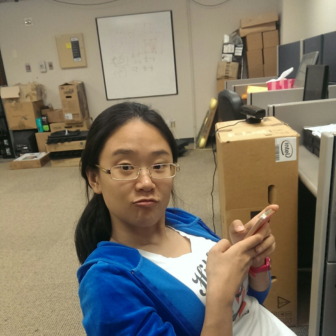
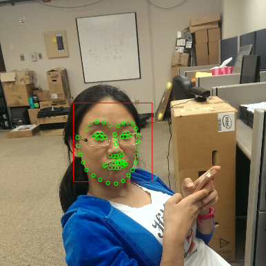
For images with side face or large expression (mostly laugh), the alignment error is much larger. The failure usually occurs in image with occlusion (case 1 and 4), extreme expression (case 2), or extreme lighting conditions (case 3). |
 |
 |
 |
 |
 |
 |
 |
| Failed case 1 | Failed case 2 | Failed case 3 | Failed case 4 |
Gallery
Please follow this link to a gallery of results.Usage
To find the face shape of an image, download the MATALB source code here, then run the following script with the provided model file in MATLAB:
model = load('model.mat');
[filename, pathname] = uigetfile({'*.jpg; *.png; *.gif; *.bmp'; '*.*'}, ...
                                 'Choose Image');
img = imread([pathname, filename]);
[box, points, succeeded] = applyModel(img, model);
if succeeded
    figure;showImageWithPoints(img, box, points);
end
Note that you need to run the above script in the folder where you put the downloaded source code
References
- Xudong Cao, Yichen Wei, Fang Wen, Jian Sun. Face Alignment by Explicit Shape Regression. In CVPR 2012.
- Xudong Cao, Yichen Wei, Fang Wen, Jian Sun. Face Alignment by Explicit Shape Regression. International Journal of Computer Vision (IJCV), Volume 107, Number 2, pages 177-190.
Author Information
This program is written by @Peihong for the final project in CSCE 625 Artificial Intelligence course in Fall 2014.
Please contact the author if you find any error/bug in the code.