It is time we work on something more sophisticated. Well, not actually that sophisticated, but complex enough compared to what we have done so far. Histogram equalization. It is a commonly used technique to save many many many poorly exposed images.

Histogram and Cumulative Distribution Function

First of all, what exactly is a histogram? Basically it is a statistics telling us about the distribution of the pixels values in a given image - how many pixels are bright, how many are dark, etc.

Let's consider a grayscale image for the moment. We know that there are typically 256 gray scales (i.e. pixel values) in such images. It is not very hard to come up with a histogram for such kind of image - we can simply count the number of pixels having different pixels values. Say we find $n_0$ pixels have gray scale 0, $n_1$ pixels have value 1, ..., $n_i$ pixels have value $i$, and so on and so on. After counting the pixels of all 256 possible gray scales, we get ourselves a histogram! Easy huh?

We can also think of the creation of a histogram as a classification of pixels according to their values, and the histogram is nothing more than a table recording the number of the pixels in each of the 256 groups (or more commonly, 'bins'). Therefore, a histogram provides a description of the pixel value distribution in an image - how many pixels are bright, how many pixels are dark, and how many mid-tone pixels, etc. This is very useful for us to design image processing algorithms because we can use it as a compact representation of an image (think about 1 million pixels versus 256 numbers!). The downside is we can not get much out of a histogram if we have a complex problem to solve, since we only have a very high level (and also very vague) summary of brightness distribution over an image.

Just a side note, we don't necessarily have to use 256 bins for the counting - any number of bins, as long as it is sufficient for the application at hand, can be used. One typical case using a very small number of bins for histogram computation is color reduction, where we try to reduce the number of colors in images while maintaining their original visual appearance as much as possible.

For color images, say RGB images, things are just as straightforward. The only difference is that we have 3 channels, i.e. R, G, B channels, instead of just a single brightness channel. So what? We can just create 3 histograms for these channels and we are done! Of course, sometimes we are only interested in the brightness of an image. In those cases, we can convert the color image to a grayscale one first, and compute the histogram for the grayscale image. How do we convert a color image to a grayscale one? Simple! We can use a rough estimation with the equation below: $$ l = 0.299 \times r + 0.587 \times g + 0.114 \times b $$

var filters = {
    grayscale : function( src ) {
        return src.map(
            function(r, g, b, a) {
                var lev = Math.round(r * 0.299 + g * 0.587 + b * 0.114);
                return new Color(lev, lev, lev, a);
            }
        );
    }
};

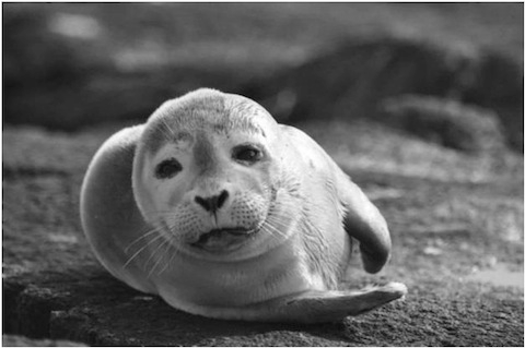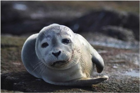
Source Image	Converted Grayscale Image

A conversion using the above equation works just fine, and we are ready to get compute a histogram for any image! The computation of histogram is pretty straightforward:

// build histogram of specified image region
function histogram(img, x1, y1, x2, y2, num_bins) {
    if( num_bins == undefined )
        num_bins = 256;
    var h = img.h, w = img.w;
    var hist = [];
    var i, x, y, idx, val;
    // initialize the histogram
    for(i=0;i<num_bins;++i)
        hist[i] = 0;
    // loop over every single pixel
    for(y=y1,idx=0;y<y2;++y) {
        for(x=x1;x<x2;++x,idx+=4) {
            // figure out which bin it is in
            val = Math.floor((img.data[idx] / 255.0) * (num_bins-1));
            ++hist[val];
        }
    }
    return hist;
}

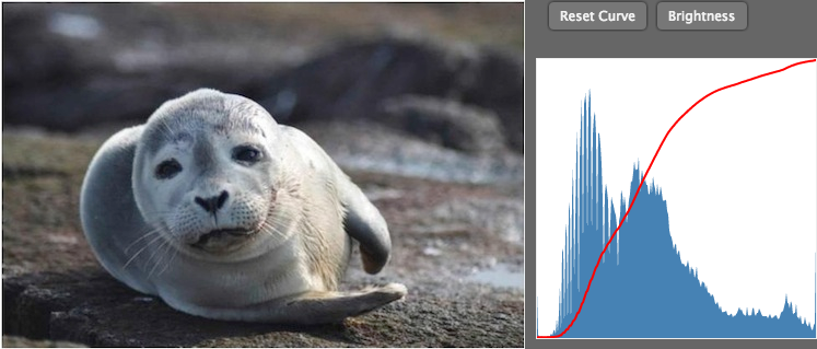Seal and its histogram

Yes, the jagged blue area is the histogram. The horizontal axis represents the pixel values, and the vertical axis is their frequency. Not so shabby, right? You may ask what on earth is the red curve in the plot, we will get to that in a bit.

Let's first formalize the definition of the histogram. The histogram can be viewed as a function of pixel values $h(p): R \to R$. This function maps a given pixel value $p$ to its frequency, $\frac{n(p)}{N}$, in the entire image. Here we use $n(p)$ for as the number of pixels having a brightness value $p$, and $N$ as the total number of pixels in an image. Since the number of pixels in an image is a normalizing factor, we can also just use $n(p)$ as the frequency as well.

Now what exactly is the red curve? It is the so-call cumulative distribution function(CDF). Don't be scared away by its long name, it is just a partial sum of the histogram we just build: $$c(p) = \sum_{i=0}^p n(i)$$ Yes, $c(p)$ means the number of pixels with a value smaller or equal than $p$. So $c(0)$ means the number of the pure black (0, 0, 0) pixels, while $c(255)$ equals to the total number of pixels. If we are using a normalized version of histogram, we will have

$$c(p) = \frac{1}{N} \sum{i=0}^p n(i) = \sum\{i=0}^p h(i)$$

In this case, we have $c(256)=1$. Now let's take a look at the histogram we just build. For display purpose the histogram is scaled slightly differently, but the CDF is normalized with the total pixel number. The vertical axis has a range of [0, 1], while the horizontal axis has a range of [0, 255]. Things look just about right.

Histogram Equalization

Now that we have the histogram built and displayed, what then? What can all these vertical bins do? Let's consider the badly exposed image below.

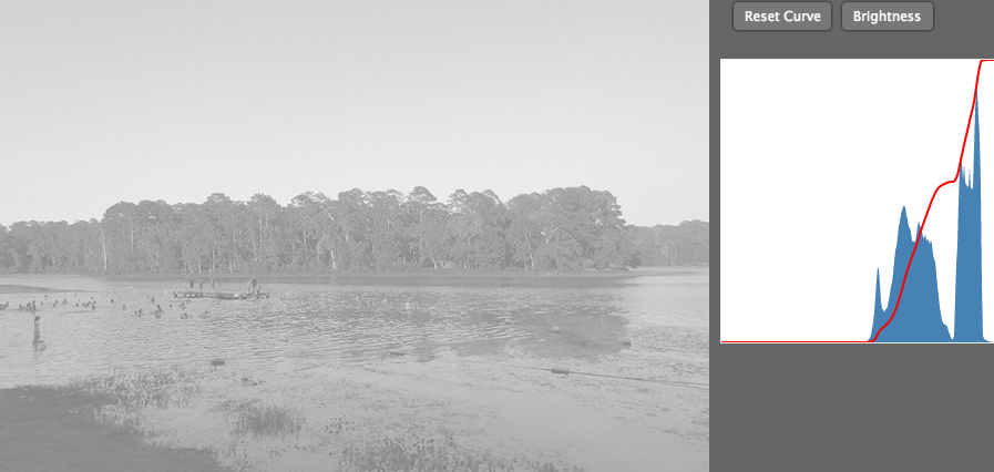Badly Exposed Image

Not cool. Everything just look so washed. We've got to do something to rescue it.

And here comes histogram equalization. The histogram of the image above is totally skewed. All the interesting pixel values are well above 128 roughly -- this means about we wasted roughly half of the useful pixel values! That's exactly the reason this image looks so bad. And the way to make it better seems obvious: just distribute the pixel values better, or even better, distribute them evenly across all available levels. That's right, make use of all available levels so that the differences among pixels values are better presented and the details of the image are better visible.

This is the so called histogram equalization - to make the pixels distributed "equally" to different brightness levels while maintaining the visual appearance of the image. The key to histogram equalization is to maintain visual appearance. We can easily make the histogram any shape we want, but that would not work because the visual appearance of the image would also be completely changed. To preserve visual appearance, we need to keep the relative relationship among pixels unchanged. That is, if a pixel $pi$ has a larger value than $pj$, it should still have a large value after histogram equalization.

To achieve this, we need to scale each pixel value by some factor. The factor can be determined by applying the equalization condition: after equalization, the total number of pixels with value smaller or equal to $p$ should have a new value $p'$ such that $$\frac{p'}{255} = c(p)$$ The meaning of this equation is apparent: if the fraction of pixels with value smaller or equal to $p$ is $c(p)$, then all value $p$ pixels should have a new value $p'$ that is proportional to $c(p)$. That is, $p' = const \cdot c(p)$. Considering there are in total 256 levels of brightness and the minimum brightness is 0, the constant must be 255.

This is a very intuitive solution, because we do want to assign a smaller value to low brightness pixels and larger values to high brightness pixels. This is guaranteed with the equation above since $c(p)$ is monotonic increasing with $p$. The equation also guarantees that the pixel values distribution in the new image is equalized. The reason is that the CDF of the new image satisfies $$c(p') = c(p) = 255\cdot p'$$ $c(p') = c(p)$ because the ratio of pixels smaller or equal than $p'$ in the new image is exactly the same as the ratio of pixels smaller or equal than $p$ in the original image.

A linear relation! We've got an even distribution of pixel values! Well, not exactly even distribution due to the discrete nature of the pixel values, but it is close enough to even distribution. The image below verifies this.

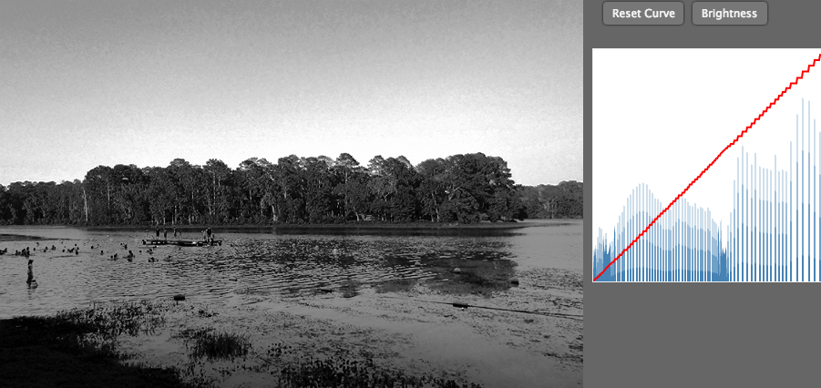Histogram Equalized Image