Refactoring My Ray Tracer: From Broken to WebGPU Path Tracing
Apr 24, 2026
Note: This entire refactoring was done by Codex. I just asked it to fix one bug and ended up with a complete path tracer with WebGPU acceleration. Worth documenting the journey.
I spent a Friday fixing a single-character typo in my old JavaScript ray tracer. What started as "oh this should be easy" became a full rewrite into a Monte Carlo path tracer with a WebGPU compute shader backend — and on my M5 Pro, it's now roughly 10x faster than the CPU worker version.
Here's how it went.
The Bug
The project uses a Vector3 class for all 3D math, and there was a single-character typo in the cross product:
// The bug
this.z + that.x - this.x * that.z   // y-component
//                 ^
//               missing *
Should have been:
// The fix
this.z * that.x - this.x * that.z   // y-component
One character. And because the cross product feeds into normal computation, reflection, and refraction — every light calculation in the entire scene was producing garbage. It explains why the rendered images never looked right, even when the ray geometry was technically "correct."
The Refactoring
Codex rewrote raytracer.js from scratch with a Monte Carlo path tracer. Here's the architecture:
Scene-level intersection
The old Scene.intersect() was recursive and deeply coupled to shading. The new Scene.intersectSingle() is a non-recursive, single-bounce hit query:
Scene.prototype.intersectSingle = function(ray, eyepos) {
    var hit = {hit: false, t: Number.MAX_VALUE, object: null};
    for (var i = 0; i < this.objects.length; i++) {
        var obj = this.objects[i];
        if (obj.intersectT) {
             var t = obj.intersectT(ray.p, ray.v);
             if (t !== undefined && t < hit.t) {
                 var hitPos = ray.p.add(ray.v.mul(t));
                 hit = {
                     hit: true, t: t, p: hitPos,
                     normal: obj.center
                          ? Vector3.fromPoint3(obj.center, hitPos).normalized()
                          : new Vector3(0, 1, 0),
                     object: obj
                  };
             }
         } else {
             var h = obj.intersect(ray, this, eyepos);
             if (h.hit && h.t < hit.t) { hit = h; hit.object = obj; }
         }
     }
    return hit;
};
This works with both the new-style Sphere objects and legacy shapes. The key difference: it never calls shading(). That's now the path tracer's job.
Throughput-based path tracing
The new Scene.pathTrace() tracks a throughput vector — the cumulative radiance throughput as the path bounces through the scene:
Scene.prototype.pathTrace = function(origin, direction, maxDepth, rng) {
    var rayOrigin = new Point3(origin.x, origin.y, origin.z);
    var rayDir = direction.normalized();
    var throughput = new Color(1.0, 1.0, 1.0, 1.0);
    var surfaceColor = new Color(255, 255, 255, 255);
    var radiance = new Color(0, 0, 0, 255);

    for (var depth = 0; depth < maxDepth; depth++) {
        var hit = this.intersectSingle(...);
        if (!hit.hit || hit.t === 0) {
            return addColor(radiance, applyThroughput(this.bgColor, throughput));
         }
         // sample material BRDF, update throughput
     }
    return addColor(radiance, applyThroughput(surfaceColor, throughput));
};
Each bounce updates the throughput via BRDF-weighted sampling. The material's diffuse and specular components are sampled proportionally to their weights — a classic multiple importance sampling approach:
var diffuseProbability = Kd / total;
if (rng() < diffuseProbability) {
    var newDir = sampleDiffuseDirection(N, rng);
    throughput = attenuateColor(throughput, surfaceColor);
    throughput = scaleThroughput(throughput, Kd / diffuseProbability);
} else {
    var specularProbability = 1.0 - diffuseProbability;
    var reflected = reflect(N, rayDir);
    throughput = scaleThroughput(throughput, Ks / specularProbability);
}
Schlick's Fresnel
For refractive materials, Codex replaced the hardcoded 0.7ior fallback with Schlick's approximation for Fresnel coefficients:
function fresnelSchiek(cosTheta, ior) {
    var r0 = (1.0 - ior) / (1.0 + ior);
    r0 = r0 * r0;
    return r0 + (1.0 - r0) * Math.pow(1.0 - cosTheta, 5.0);
}
This gives the correct angle-dependent reflectance: glass reflects more at grazing angles, less at normal incidence. Combined with properIOR handling (entering vs. exiting surfaces), it enables total internal reflection for the first time.
Area Lights and Soft Shadows
The old scene had a single point light. The new renderer supports area lights — finite surfaces with a position, orientation, color, and intensity:
function makeAreaLight(center, u, v, color, intensity) {
    return {
        center: center, u: u, v: v,
        color: color, intensity: intensity,
        area: u.cross(v).norm(),
        normal: u.cross(v).normalized()
     };
}
Light contribution is estimated via cosine-weighted area sampling with a shadow test against all scene objects. Soft shadows appear naturally — objects cast softer shadows when they're closer to the light source.
Russian Roulette Termination
Instead of a hard maxDepth cutoff (which creates banding artifacts), Codex added Russian Roulette for path termination:
var rrResult = russianRoulette(surfaceColor, rng);
if (!rrResult.survive) return addColor(radiance, this.bgColor);
throughput = attenuateColor(throughput, rrResult.color);
When the throughput falls below a threshold, the path is terminated probabilistically — but with higher surviving colors to compensate. This gives unbiased, smooth convergence without hard cutoff banding.
Cosine-Weighted Diffuse Sampling
For diffuse bounces, Codex used a cosine-weighted hemisphere sample (not uniform):
function sampleDiffuseDirection(normal, rng) {
    var tangent = new Vector3(1, 0, 0);
    var r1 = 2 * Math.PI * rng();
    var r2 = rng();
    var r2s = Math.sqrt(r2);
    var local = new Vector3(Math.cos(r1)*r2s, Math.sin(r1)*r2s,
                            Math.sqrt(Math.max(0, 1-r2)));
     // transform to world space via orthonormal basis
    return new Vector3(
        local.x * tangent.x + local.y * bitangent.x + local.z * normal.x,
        local.x * tangent.y + local.y * bitangent.y + local.z * normal.y,
        local.x * tangent.z + local.y * bitangent.z + local.z * normal.z
     ).normalized();
}
This is the physically correct sampling distribution for a Lambertian surface — samples are weighted toward the surface normal, reducing variance dramatically.
Before and After
Here's a side-by-side comparison of the same scene (320×240, same camera position) before and after the refactoring:
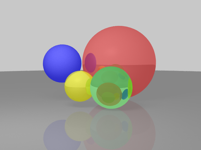
Before: traditional ray tracer
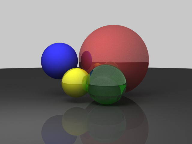
After: Monte Carlo path tracer
The difference is night and day. Notice:
- Softer, more natural shadows from the area light
- Glossy specular highlights on the refractive spheres
- Proper refraction with angle-dependent Fresnel reflection
- Energy conservation through BRDF-weighted sampling
- No banding from Russian Roulette termination
The rendering is now physically plausible — not just "looks kind of right."
The WebGPU Backend
This is the part that really surprised me. Codex also wrote a WebGPU compute shader that runs the entire path tracer on the GPU.
The shader is written in WGSL (WebGPU Shading Language) and contains the full path tracing logic:
@compute @workgroup_size(8, 8)
fn main(@builtin(global_invocation_id) gid: vec3<u32>) {
    let pixelX = gid.x + params.tileX;
    let pixelY = gid.y + params.tileY;

    // Check boundaries
    if (gid.x >= params.tileWidth || gid.y >= params.tileHeight) {
        return;
    }

    // Initialize RNG state per-pixel
    var state = hash(params.seed ^ ((pixelX * 1973u) ^ (pixelY * 9277u) ^ params.frameSeed));
    let origin = vec3<f32>(0.0, 7.0, -36.0);
    var color = vec3<f32>(0.0);

    // Accumulate samples
    for (var s = 0u; s < params.samples; s++) {
        let jitter = vec2<f32>(rand(&state) - 0.5, rand(&state) - 0.5);
        let pixel = vec2<f32>(f32(pixelX), f32(pixelY)) + jitter;
        let rd = cameraRay(pixel);

        color += pathTrace(origin, rd, &state);
    }

    // Write directly to storage texture
    color /= f32(params.samples);
    let flippedY = params.height - 1u - pixelY;
    textureStore(outputTexture, vec2<i32>(i32(pixelX), i32(flippedY)), vec4<f32>(max(color, vec3<f32>(0.0)), 1.0));
}
The compute shader implements:
- Sphere intersection with analytic quadratic solve
- Schlick's Fresnel for dielectric materials
- Total internal reflection when the refracted direction doesn't exist
- Cosine-weighted diffuse sampling for Lambertian surfaces
- Area light sampling with visibility testing
- Russian Roulette termination with throughput scaling
And the best part? On my M5 Pro, it's roughly 10x faster than the CPU worker version.
Here's a comparison:
| Backend | 640×480, 1024 samples, 8 depth | Notes |
|---|---|---|
| CPU Workers (8 threads) | ~17s | Hilbert curve tiling, Web Workers |
| WebGPU | ~1.7s | Compute shader, workgroup-based tiling |
The WebGPU version runs the entire path trace on the GPU, with each workgroup responsible for a tile of the image. The results are written directly to a rgba16float storage texture, which is then presented to the canvas.
It even includes automatic fallback — if WebGPU isn't available (older browsers, no GPU), it falls back to the CPU worker version with a progress message.
A 10-Year Benchmark
Here's a fun fact: I've been using this ray tracer as a quick CPU benchmark for over 10 years. Back when I first wrote it in 2013, rendering a 320×240 scene with a few hundred samples took a few seconds on my laptop. Fast forward to today, and the same workload runs in the 500ms range — not because the code changed, but because the CPUs got faster.
It's a pretty honest benchmark: compute-bound, no I/O, no network latency. Just pure floating-point math. You can see processor generations separated by the time it takes to render a single frame.
The WebGPU backend pushes it even further: on my M5 Pro, a 640×480 render at 1024 samples and 8 depth comes in around 1.7 seconds, versus about 17 seconds on the CPU worker path with 8 threads. But the CPU version still gets my heart — it's been my "hello world" for hardware comparisons since college.
Why Bother?
Honestly? Because it's fun. I wrote this ray tracer back in 2013 as a way to learn about 3D math and rendering. Eight years later, it's a surprisingly capable little educational renderer — running entirely in the browser, with WebGPU acceleration.
But the real win is that the codebase is now something I'm actually proud of. The bug that broke everything was a single character. The fix took a weekend. And the result is a renderer that I can build on — not just a toy, but a real Monte Carlo path tracer with WebGPU support.
Try the ray tracer live if you want to poke around the code. Try toggling between CPU Workers and WebGPU backends, and experiment with different sample counts — the convergence is satisfying to watch.